Example: Multiplayer Perceptron Binary Classifier

Data

Datasets & Templates

Task: A bank have seen an unsual churn rate and try to find out and address the reasons why customers leave the bank.
Data: Dataset of 13 different values of 10.000 customers, including if a customer recently left the bank.

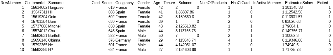
The (fictional) data consists of the following values:

1. RowNumber: an increasing number for each customer in the list (Integer)
2. CustomerID: the unique customer identification number for each customer (Integer)
3. Surman: the customers surname (String)
4. Credit score: a score showing the credibility of a customer (Integer)
5. Geography: one of 3 different locations for the different bank locations (France, Spain or Germany)
6. Gender: one of 2 possible gender of the customer (Male or Female)
7. Age: the age of the customer (Integer)
8. Tenure: the number of years that customer has a bank account at this bank (Integer)
9. Balance: the amount of money in the customers bank account (Float)
10. NumOfProducts: the number of different products a customer (Integer)
11. HasCrCard: has the customer a credit card? (Boolean / 0 or 1)
12. IsActiveMember: has the customer recently used his account (Boolean / 0 or 1
13. EstimatedSalary: an estimation of the customers income (Float)
14. Exited: has the customer recently left the bank? (Boolean / 0 or 1)

We start creating the example by importing required packages.

# Importing the libraries
import numpy as np
import matplotlib.pyplot as plt
import pandas as pd

In a published version of this script, we would import ALL required packages right at the beginning. To increase the readability we encapsulate different parts of the code instead, including the used imports.

The next step is the import of the data, which is stored in a file called Churn_Modelling.csv, a comma seperated file with table structure. One of the easiest and most performant ways of import csv files is the use of pandas.read_csv function. By an observation, we notice that only values of column CreditScore to EstimatedSalaray may influence the customers decision. Our neural network task is to make use of these columns to predict canditates, that are willing to leave.

We load the subset of columns and call this list of vector X. We also load the last column, which is the indication if a customer has recently left the Bank to the variable y. The neural network will be trained, such that it may predict the status y by the use of X.

# Importing the dataset
dataset = pd.read_csv('Churn_Modelling.csv')
X = dataset.iloc[:, 3:13].values
y = dataset.iloc[:, 13].values

Data Encoders

The data consists of values of diffesrent types and ranges. The salary, for example, is of type float and its value about 100.000 and the geography is an enumeration with three different possible values. Since neural networks cannot make use of them, there exist functions to transform enumerations (categoricals) into numerical values: the LabelEnconder and the OneHotEncoder. Both functions are part of the sklearn.preprocessing package.

The label encoder takes categorical data and transform the categories to inceasing numbers. Since we have 2 categorical variables (Geography and Gender), we apply a label encoder to both of them seperatly.

# Encoding categorical data
from sklearn.preprocessing import LabelEncoder, OneHotEncoder
labelencoder_X_1 = LabelEncoder()
X[:, 1] = labelencoder_X_1.fit_transform(X[:, 1])
labelencoder_X_2 = LabelEncoder()
X[:, 2] = labelencoder_X_2.fit_transform(X[:, 2])

So the gender becomes 0 and 1 instead of male and female and the geography was transformed to 0, 1 and 2 from Spain, France and Germany. If there are more than 2 categories, one has to apply another function to the column, the OneHotEncoder. We apply this function to the Geography column.

onehotencoder = OneHotEncoder(categorical_features = [1])
X = onehotencoder.fit_transform(X).toarray()
X = X[:, 1:]

It transforms our column with 3 categorical values to 3 boolean columns. This could be named isfrance, isspain _and isgermany_. While the original column is removed by the function, the 3 boolean columns are attached LEFT at the matrix. Since we would run into the dummy variable trap we have to remove one of the 3 columns and we removed the first one. The OneHotEncoder also transforms the type of our matrix to float, which is required by the network.

Scaling

To test for overfitting we split our data into a training set and a test set. The is easily done by the train\_test\_split function of sklearn.model\_selection. We split out data into 80% training and 20% test data.

# Splitting the dataset into the Training set and Test set
from sklearn.model_selection import train_test_split
X_train, X_test, y_train, y_test = train_test_split(X, y, test_size = 0.2, random_state = 0)

Neural networks only work with scaled numerical data, such that the different input variables equal in mean and standard deviation. The normalization is executed by the StandardScaler class of sklearn.preprocessing. Since the test data should be ne part of any parameter estimation, the standard StandardScaler get only fit by the training data. The transformation is then seperatly applied to the test set, as you would do it with new data.

# Feature Scaling
from sklearn.preprocessing import StandardScaler
sc = StandardScaler()
X_train = sc.fit_transform(X_train)
X_test = sc.transform(X_test)

The data is now transformed and read to process by a neural network.

Creating the neural network

Finally we create the neural network by using keras. A keras netzwork is usually initialized by creating a Sequential Instance. The different layers are added by its add function, with the initialized Layer Object.

# Importing the Keras libraries and packages
import keras
from keras.models import Sequential
from keras.layers import Dense

# Initialising the ANN
classifier = Sequential()

# Adding the input layer and the first hidden layer
classifier.add(Dense(units = 6, kernel_initializer = 'uniform', activation = 'relu', input_dim = 11))

# Adding the second hidden layer
classifier.add(Dense(units = 6, kernel_initializer = 'uniform', activation = 'relu'))

# Adding the output layer
classifier.add(Dense(units = 1, kernel_initializer = 'uniform', activation = 'sigmoid'))

# Compiling the ANN
classifier.compile(optimizer = 'adam', loss = 'binary_crossentropy', metrics = ['accuracy'])

In This example we only use Dense layers, representing fully connected layers as shown in the introduction. Each layer has different parameters. The most important parameters are:

• units - the number of nodes in the layer
• activation - the nodes activation function
• kernel_initializer - each weight is initialized by a configured function, in most cases this is uniform
• input_dim - only used in the first layer to specify the number of input variables

We create a network consisting of 2 hidden layers of 6 neurons each and a output layer of one node. We use the sigmoid function to predict a score between 0 and 1. Afterwards we will use a treshold of 0.5 to transform the score into a binary prediction. Since our matrix holds 11 columns, we initialize the number of input variables with 11.

At the end we compile our network by calling the compile function and tell the compiler to use the widely used adam optimizer, a binary crossentropy loss function and let it show the accuray metric during the process.

In the next step we'll fit our training data to the network by 100 iterations (epochs) and a batch size of 10.

# Fitting the ANN to the Training set
classifier.fit(X_train, y_train, batch_size = 10, epochs = 100)

We previously split the data into 8000 training samples and the training process will produce the following output

Epoch 1/100
8000/8000 [==============================] - 1s - loss: 0.4950 - acc: 0.7950       
Epoch 2/100
8000/8000 [==============================] - 0s - loss: 0.4305 - acc: 0.7960     
Epoch 3/100
8000/8000 [==============================] - 0s - loss: 0.4265 - acc: 0.7960     
Epoch 4/100
8000/8000 [==============================] - 0s - loss: 0.4219 - acc: 0.7990
...
Epoch 98/100
8000/8000 [==============================] - 0s - loss: 0.3403 - acc: 0.8600     
Epoch 99/100
8000/8000 [==============================] - 0s - loss: 0.3408 - acc: 0.8604     
Epoch 100/100
8000/8000 [==============================] - 0s - loss: 0.3405 - acc: 0.8596

Each line represents one iteration (epoch) of the fitting process with sample count (8000/8000), running time. The metrices are the loss value of the loss function and the measured accuracy (fraction of correct predictions).

Prediction and Evaluation

To test our network with unseen data, we apply our classifier to our test set and create the confusion matrix.

# Making predictions and evaluating the model

# Predicting the Test set results
y_pred = classifier.predict(X_test)
y_pred = (y_pred > 0.5)

# Making the Confusion Matrix
from sklearn.metrics import confusion_matrix
cm = confusion_matrix(y_test, y_pred)

The confusion matrix contains the number of true/false positive/negative predictions.